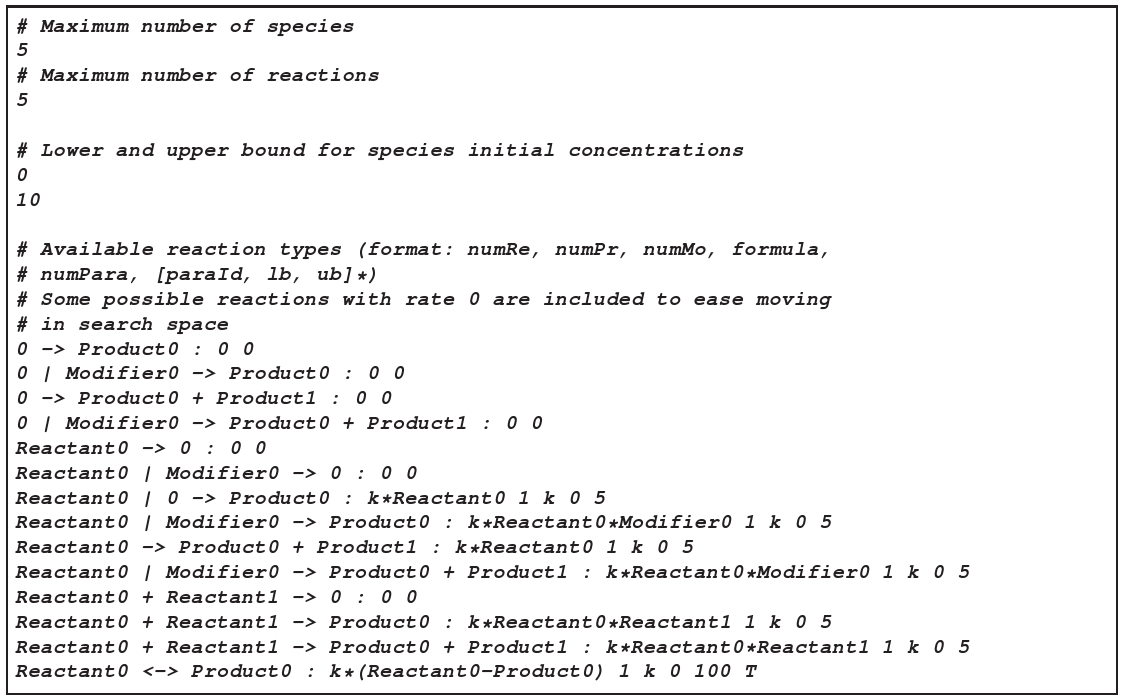
figure 3
buildingblocks.txt
(figure 3). As you can see, we only use mass-action kinetics here. We also specify boundaries for the parameters, which helps to avoid numerical problems in the integration when the time-scales become too separated.input1
andinput2
(more should be used, but this is not done here due to space constraints). We will measure the concentration ofoutput
at four timesteps of 2.0 seconds each, ignoring the first one (offset). Since the input is only to be specified at t = 0, we put a ’*’ in front of its concentration. We do not want to use Akaike’s Information Criterion to modify the fitness (noAIC
), and we want to have a mass-conserving network (penalties for non-massconservance and size).options.txt
(see figure 5). In this case, we choose to use a population size of 20, producing 80 offspring in a overlapping fashion, such that selection acts on 100 individuals. The population is then refilled by mutations and crossover on the survivors. All survivors are selected by elitist selection. Every tenth offspring should be produced by crossover between survivors. This is a very strong selection pressure, so it will only be successful in simple cases such as this example. In each fitness evaluation, the model parameters are be improved in a (1,5)-ES for 15 generations. Since we use default filenames for all files, we can call the SBMLevolver without command-line arguments.| Turn | Best | Avg | Diff1 | Diff2 | Species | Reactions | |
|---|---|---|---|---|---|---|---|
| 1 | 6.431398 | 26.97341 | 7.960000 | 5.640000 | 3.200000 | 4.800000 | |
| 2 | 0.084014 | 8.160019 | 9.840000 | 6.480000 | 3.800000 | 6.600000 | |
| 3 | 0.002412 | 4.835043 | 13.98000 | 7.720000 | 4.600000 | 8.900000 | |
| 4 | 0.002412 | 3.037237 | 16.78000 | 8.660000 | 5.300000 | 11.400000 | |
| 5 | 0.001200 | 0.912607 | 16.54000 | 9.440000 | 5.800000 | 12.200000 | |
| 6 | 0.000758 | 0.007115 | 9.980000 | 9.180000 | 5.900000 | 12.100000 | |
| 7 | 0.000246 | 0.001053 | 12.52000 | 9.240000 | 6.000000 | 13.700000 | |
| 8 | 0.000098 | 0.000412 | 15.76000 | 9.340000 | 5.900000 | 15.700000 | |
| 9 | 0.000088 | 0.000248 | 17.84000 | 9.620000 | 5.700000 | 16.400000 | |
| 10 | 0.000057 | 0.000136 | 20.82000 | 10.46000 | 6.300000 | 17.600000 | |
| 11 | 0.000035 | 0.000107 | 25.52000 | 11.18000 | 6.700000 | 20.000000 | |
| 12 | 0.000010 | 0.000053 | 24.00000 | 11.74000 | 8.100000 | 19.500000 | |
| 13 | 0.000010 | 0.000047 | 29.48000 | 13.62000 | 8.700000 | 23.700000 | |
| 14 | 0.000010 | 0.000047 | 29.48000 | 13.62000 | 8.700000 | 23.700000 | |
| 15 | 0.000003 | 0.000035 | 33.38000 | 14.88000 | 9.000000 | 27.600000 |