User interface

In this file (default is

option.txt

), the algorithmic parameters and any other controls are given as:

These can also be accesses by calling the programm with the

-h

or

--help

option. Each parameter is given on a new line. Here is a list of all available parameter options:

Input & Output
output_file	output file (additional to stdout)
input_dir	input directory (working directory before run)
output_dir	result directory (working directory while and after run)
objective	objective function file (default: objectivefunction.txt)
bblocks	building blocks file (default: buildingblocks.txt)
first_model	initial ”seed” model file
save_every	number of generations after which to save models
num_save	number of models to save from population every save_every turn
Experiment Settings
num_pop	number of populations (default 1)
iso_time	isoluation time when using multiple populations
mu	population size (default: 10)
lambda	number of offspring (default: 100)
comma_selection	if given, comma selection is used instead of plus selection
mutation_probs	relative frequencies for the different kinds of mutations (default: 1 1 1 1 1 1 1; no mutation, add/delete species, replace reaction, add/delete reaction, duplicate species)
max_mutations	maximal number of mutations per mutation-turn (default: 1)
cross_prob	probability of crossover instead of mutation
pf_settings	population size, number of offspring, number of generations of local parameter fitter (CMA-ES-algorithm, (mu,lambda) strategy)
Termination Conditions
stop_time	time limit (in seconds)
stop_turn	iteration limit
stop_fitness	fitness to reach (default: 0.0)

The modular architecture allows the user to specify his or her own fitness function in a separate file in the directory

src/objectives

. This file then has to be included into the class

ObjectiveFunction

(just follow the way

io-table.cpp

is included now). However, a default objective function based on an input-output table is available which can readily be used. A text file

objectivefunction.txt

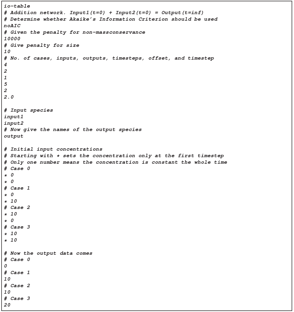
has to be provided which specifies the desired input-output behaviour of selected species in the evolved models. In the default case, fitness is then calculated as the mean square difference between the desired and the realised timecourses. An example objective function file is given in figure 4.

The evolutionary software system deals with SBML models as solution candidates for the optimisation problem. Since these can have nearly arbitrary structure, it is necessary to lay down a-priori model specifications that the optimisation process can use. This is done in the file

buildingblocks.txt

and handled in the class

BuildingBlocks

. The building-blocks specification consists of the following elements:

• The maximum number of species that can be used in the model
• The maximum number of reactions
• Lower and upper bounds for the initial concentration of each species
• A list of allowed reaction mechanisms, given in the following format (on one line):
  
  figure 3
  
  Re1 + Re2 + ... | Mod1 + Mod2 + ... -> Pr1 + Pr2 + ... : kinetic_law number_of_parameters (name lb ub)* [T]
  where (name lb ub)* denotes a series of parameter names followed by their lower and upper bounds, and the optional flag

  T

  at the end denotes transport reactions, which can involve species from different compartments (others cannot).
  The reserved names

  Reactant<num>

  ,

  Modifier<num>

  , and

  Product<num>

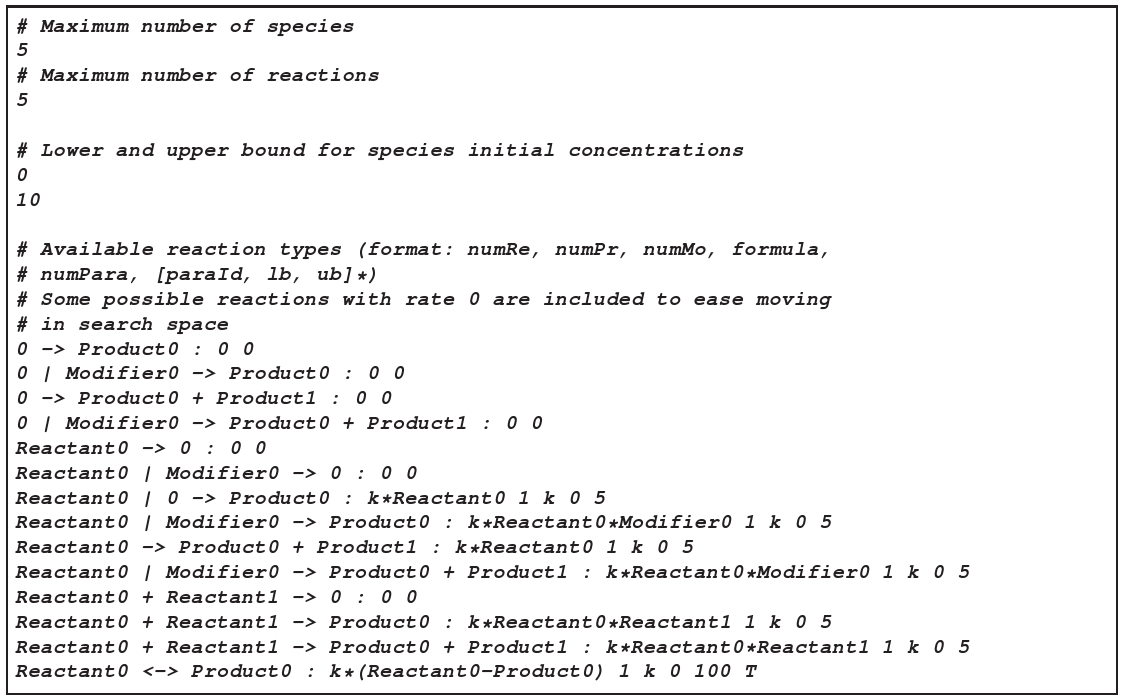
  can be replaced by arbitrary species in the evolver. This way, a mix of species-specific and general reaction mechanisms can be specified. E.g., the reaction
  Reactant0 + 02 -> Product0
  describes the oxidization of an arbitrary species, i.e. the reaction of an arbitrary species with Oxygen to another arbitrary species. An example of a

  buildingblocks.txt

  file is given in figure 3.

For the initial population, the program will load any SBML models in files of type

<modelname>.model.xml

from the current directory, and fill it up with random SBML models containing the number of species and reactions specified in the options, as well as any species required for the objective function. Also, it is possible to specify one initial starting model that is mutated once to create initial solutions (using the

first_model

option in

options.txt

). If no initial population is given, random models are created, for which the minimal and maximal size is specified in the options.

To start the evolver on a single machine, run

from the command line. By default, arguments are read from file

options.txt

. If a different options file is wanted, this has to be given directly after the call. After this, any options can be given, overriding the options specified in the optionsfile.

During the run, information about the fitness-development of the population is displayed on the screen. There are two ways to finish the program: either the pre-specified fitness, number of iterations or runtime is reached, or the user sends the signal SIGUSR1 to the process (

kill -SIGUSR1 <pid>

). After finishing, the program stores the population of the last generation in separate SBML files of the format

result_<id>_<fitness>.model.xml.

With these files, a run can be restarted from the exact point where it terminated.

Results of the evolution run are given in two ways: First, running statistics about the population are displayed, such as the best and average fitnesses, and mean numbers of species and reactions. Using the

output_file

option, this can be stored into a file and used for later evaluation. Second, the final population is stored as SBML models, which can be investigated using standard Systems Biology software tools (see list on www.sbml.org). Since the SBML_odeSolver has to be installed anyway, this program (and its associated tools such as the ParameterScanner) can be used to simulate, visualise and analyse the models.

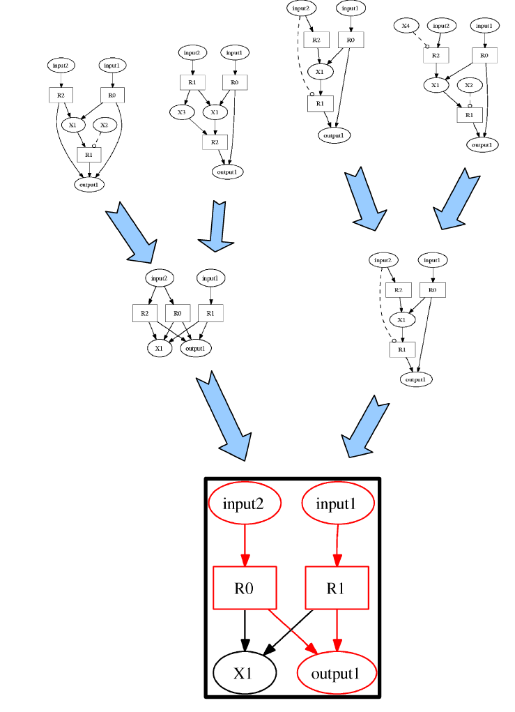
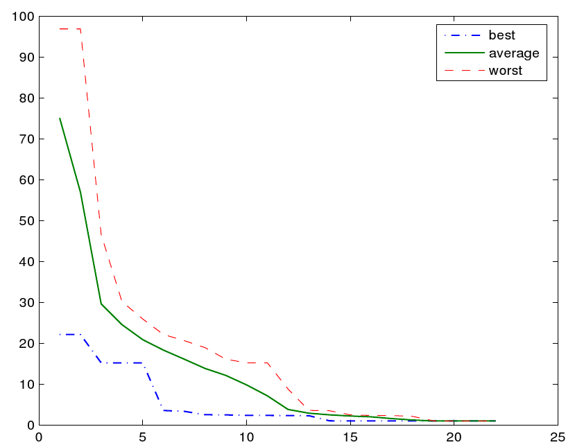
Figure 1 shows a series of snapshots from the evolution of a network capable of adding two numbers, while the corresponding fitness development is shown in figure 2. If the evolution gets stuck in a (supposedly local) optimum, one can stop and restart it with a different set of parameters, using the final population of the first run as an initial population for the second.